Tesla Cybercab Motor – Demagnetization Point-of-View

Some thoughts on the allegedly/presumably/supposed rare-earth (RE) free Tesla Cybercab motor. When I began writing this post, few details had been published other than the vague performance claims, plus an emerging consensus in the interwebs that the motor utilized ferrites.

At the moment of publishing, we seem to know, or ‘know’ – it matters not, that the machine has a nice V-plus-spoke structure (with the spokes pointing at the tip of the V if my memory serves). More importantly, it does indeed seem to be ferrite-based which is great from this post’s point of view.

So, brace yourself for a dive into the interesting world of ferrite magnets and demagnetization modelling – two seemingly unrelated topics that do actually go hand in hand.

Ferrites in general

Now, rather than going over the basics of RE magnets, supply chain concerns, and how ferrites differ, let’s jump right into the interesting stuff.

Even then, let’s get the obvious stuff out of the way. Ferrites are weaker, and by that I mean that their remanence flux density is significantly lower, typically in the range of 0.3 to 0.4 T compared to the 1.3-1.4+ T that NdFeB magnets manage. For motor topologies that produce their torque primarily via PM interaction, that translates to an equivalent reduction in torque.

Traction motors typically leverage the reluctance torque, aka the magnetic asymmetry (saliency) of the rotor. The rotor wants to align itself in such a way that the stator-excited magnetic field component travels along the rotor air, rather than having to jump over the magnet (which have a permeability close to air).

Meaning, the drop in peak torque (for a drop-in replacement) won’t be as significant as the remanence alone would suggest.

Conductivity

Unlike Neodymium magnets, ferrites are electrically non-conductive which is a huge plus for them. No eddies, significantly reduced rotor losses, easier thermal management.

Demagnetization

The bigger problem is demagnetization resistance, though.

The intrinsic coercivity (HcJ) of a magnet material is typically used as a shorthand for its demagnetization resistance. Some math follows, sorry.

The flux density in a permanent magnet can be expressed with something like (looking along the axis of magnetization alone)

   

where is the…magnetic polarization if I remember right. I always tend to mix it up with magnetization.

Now, for moderate external fields , the polarization follows, with some abuse of notation, the linear relationship

   

Here, the number if obviously rarely exact, but it is generally in the right ballpark. Now, combining the two equations yields the more-familiar equation

   

Now, back to the intrinsic coercivity. It is defined at the field at which equals zero. Based on the linear approximation, we’d need an absolutely humongous field to reach that.

That would be great for demagnetization resistance, but sadly it is rarely the case. Instead, the behaviour follows something like the plot below, the red curve. Which, by the way, follows a very simply one-parameter exponential model from EMDtool, which I think is quite fine for most purposes.

The dependency is linear for modest values of , but once we get close-enough HcJ, it experiences a sharp drop.

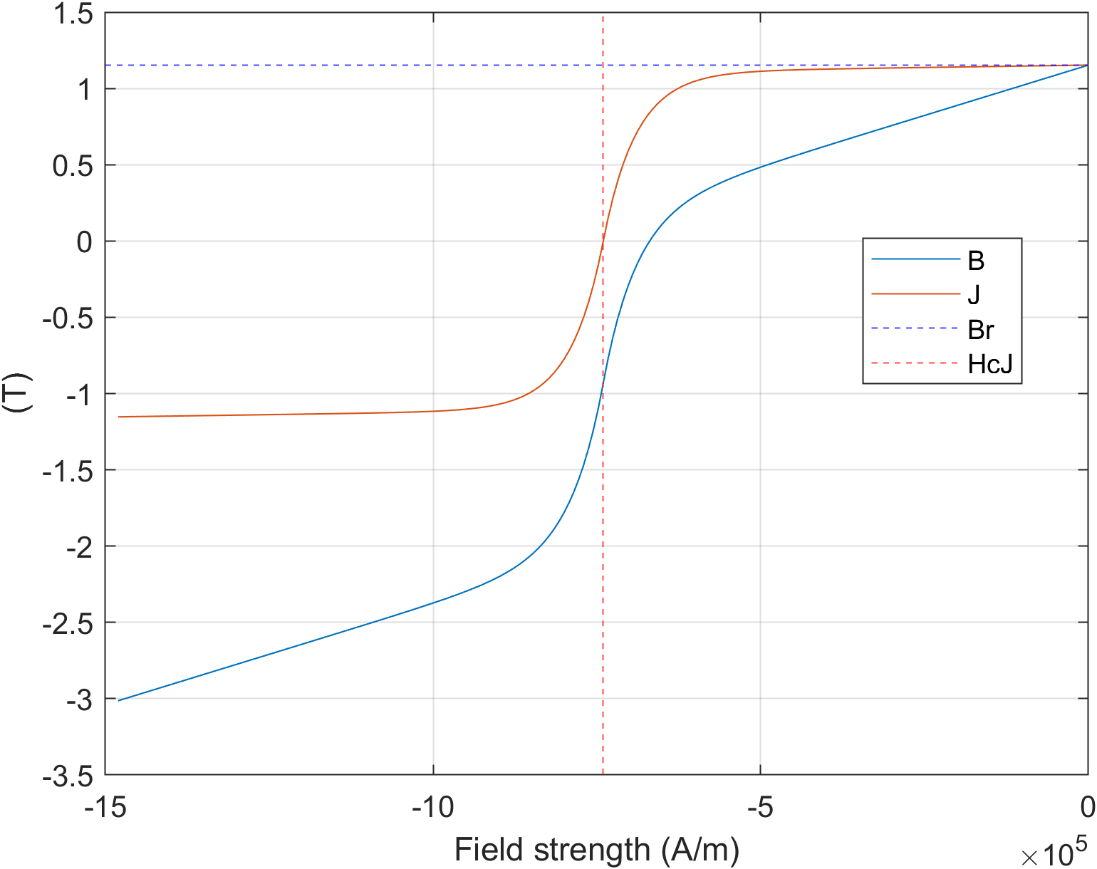
Now, if were simply nonlinear, things would be fine. But, you know that magnets can get demagnetized and this is where the effect comes from. Or where it can be seen, at least.

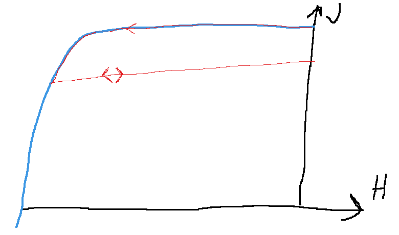
Specifically, if reaches a part of the curve where it’s no longer clearly (or nearly) linear, it doesn’t return along the same curve. A common approximation is to assume that returns – once the magnetic field is increased again – along a linear recoil curve as in the Paint art below.

The thick blue curve is the initial, or datasheet, or non-damaged curve, while the thinner red curve visualizes what happens when we first move left, dip below the knee point, and then recoil back up in terms of or the flux density. The double arrow on the last part denotes the assumption that we now have a new linear range we can move on, at a reduced level of magnetic polarization. Obviously, our knee point has now been transformed into a sharp kink rather than the original smooth transition – this is a limitation of the simple linear approximation.

Implications for traction motor use

Demagnetization is obviously something to be avoided in traction motors. And, well, any motor really, but traction motors are a rather challenging environment. The C-powers that be want to quote a this-and-that acceleration, and for that you need torque. You do need torque for regular driving, too, but it’s typically a smallish fraction of the peak 0-to-100 (or 0-to-60 for my imperial-unit pals) torque, even on a moderate uphill.

And sadly, peak torque tends to be harsh on the magnets. Deep field-weakening can be, too, and is commonly quoted, though in my experience it’s the peak torque that is often the hardest.

And ferrites are rather crap at not getting demagnetized. While Neodymium magnets typically have an intrinsic coercivity (yes I know it’s the knee point that really counts, but HcJ is a good-enough proxy for casual discussion) in the range of 1 to 2 thousand kiloamps per meter, depending on how many minefuls of dysprosium you dope them with, Ferrites will be lucky to hit 250.

Meaning, it’s very easy to demagnetize ferrites in a vehicle application. How bad it’ll actually be – well that brings us to our next topic.

Demagnetization analysis, simple to advanced

First and foremost, demagnetization is not a bulk phenomenon. Each bit of magnet tracks its own history, meaning some parts of a magnet might be damaged while others are just fine. Thus, demag risk normally can’t be evaluated with a pen-and-paper equations. You’ll get something out of them, true, but they typically only scream warning at a very extreme case.

In practice, FEA is the de-facto standard tool. In the simplest case, magnets are modelled as linear reversible materials – I would estimate this is the case for 95-98 % of the time in my own work. It’s easy to set up, the analysis runs somewhat faster though the difference in EMDtool is not very significant, and you don’t have to worry about the history dependence popping up in unintended places.

Furthermore, this type of analysis provides a nice safety check. A common practice is to log down the magnetic field component anti-parallel to the remanence direction – what I like to call the demagnetizing field. You can extract the highest value across the entire PM volume and over the entire range of time-steps simulated, if you wish a single qualitative figure. Or, you can visualize the highest value across the time-steps as a function of the position, to get a nice colorful C-suite-friendly plot that is hopefully mostly blue, or whatever your ‘good’ color happens to be.

Indeed, if the logged values are comfortably far from the knee point – more about the definition of ‘comfortable’ later – things are most likely fine.

The opposite case, seeing some bad values, typically requires some further study. For that purpose, an actual irreversible model of magnetization is needed. After all, everything the ‘bad’ values tell us is that we have strayed beyond the validity range of the model (the linear range) – the model can’t accurately predict the behaviour outside its own range.

I have personally seen the linear-reversible model predict demagnetization across one third of a magnet volume, but once you plug in a reversible model, all the harm is actually concentrated in a small volume near the magnet corner. I don’t claim to fully understand why that is the case; it’s obviously a complex interaction of the magnet material with itself and the external field.

But yeah, for more reliable results, a reversible model is needed.

Types of analysis

Once we have a reversible model in hand, there a few ways we can use it.

The simplest one is to just perform a single simulation of an operating point, or a scenario. That immediately gets us some measure of demagnetization, be it the magnet volume that has suffered at least some damage, or the maximum damage (in terms of lost remanence, for instance) incurred across the entire magnet volume.

That alone tells us relatively little, however, as not all magnet volume is made the same. We could cut off a large chunk of a corner, commonly, with few ill effects, but take the same from the middle and suddenly things get noticeably worse.

So, a good practice is to follow the demagnetizing scenario with a regular operating point. You can compare the torque reached with a given current before and after damage, for instance, or determine the current needed to reach a given torque. It could technically happen that the initial damage triggers a cascade of further demagnetization, even under regular operation, so analyzing at least two periods of the torque (a term I just came up with, meaning the period over which the torque should be periodic; 1/6th of an electrical period for regular distributed-wound synchronous machines; something horrible for anything else) and seeing if there is a downward trend.

Finally, no text about traction motors and demagnetization would be complete without a mention of active short circuits or ASCs. ASC refers to an intentional three-phase short-circuit at the inverter terminals, for instance to protect the inverter and the battery pack from an overvoltage in the case of losing synchronization / rotor angle signal / motor control in general at a high speed.

Far too often, short-circuit analysis simply considers the steady state current, approximately regardless of the speed. Reality is often vastly more violent than this.

Obviously, transient analysis with all bells and whistles enabled is the choice for best results. For instance, induced eddies in the permanent magnets or the shaft or eddy shield or any conductive bodies can have noticeable effect on the results.

For something closer to a rule-of-thumb analysis, and I hope you include FEA-based lookup tables in your definition of a thumb, comes from Martin (thank you again for pointing this out to me!). We have the pre-short operating point , and the steady state current .

Now, once we short all three terminals, the phase flux linkages approximately freeze into their values just before the short. In the dq-frame, this means that the current vector will start drawing a circle. This circle is centered on and begins its travel from . In reality, it will be closer to decaying spiral, but a circle is a good approximation for most cases. This is particularly true for larger machines, where inductances typically dominate over the resistance (which is responsible for the circle decaying in the first place).

Often neglected

As mentioned, demagnetization is typically analyzed by only considering the field component anti-parallel to the remanence direction. Sadly, reality is disappointing in this respect, too, and the perpendicular field component also plays a role.

The last time I reviewed this-which admittedly was several years ago-there was relatively little published about the topic. The best I could find was from Dr. Sami Ruoho’s thesis. Using a pulse magnetization tester, he measured the magnetic field strength required to demagnetize the magnet by 10 percent.

The results are visualized below with the black circles, plotted with respect to the inclination angle and normalized versus the intrinsic coercivity. For instance, at 90-degree inclination so a perfectly perpendicular field, approximately is needed.

While this is a lot, oftentimes, it is a significantly harsher limit than the no demagnetization ever predicted by the typical analysis.

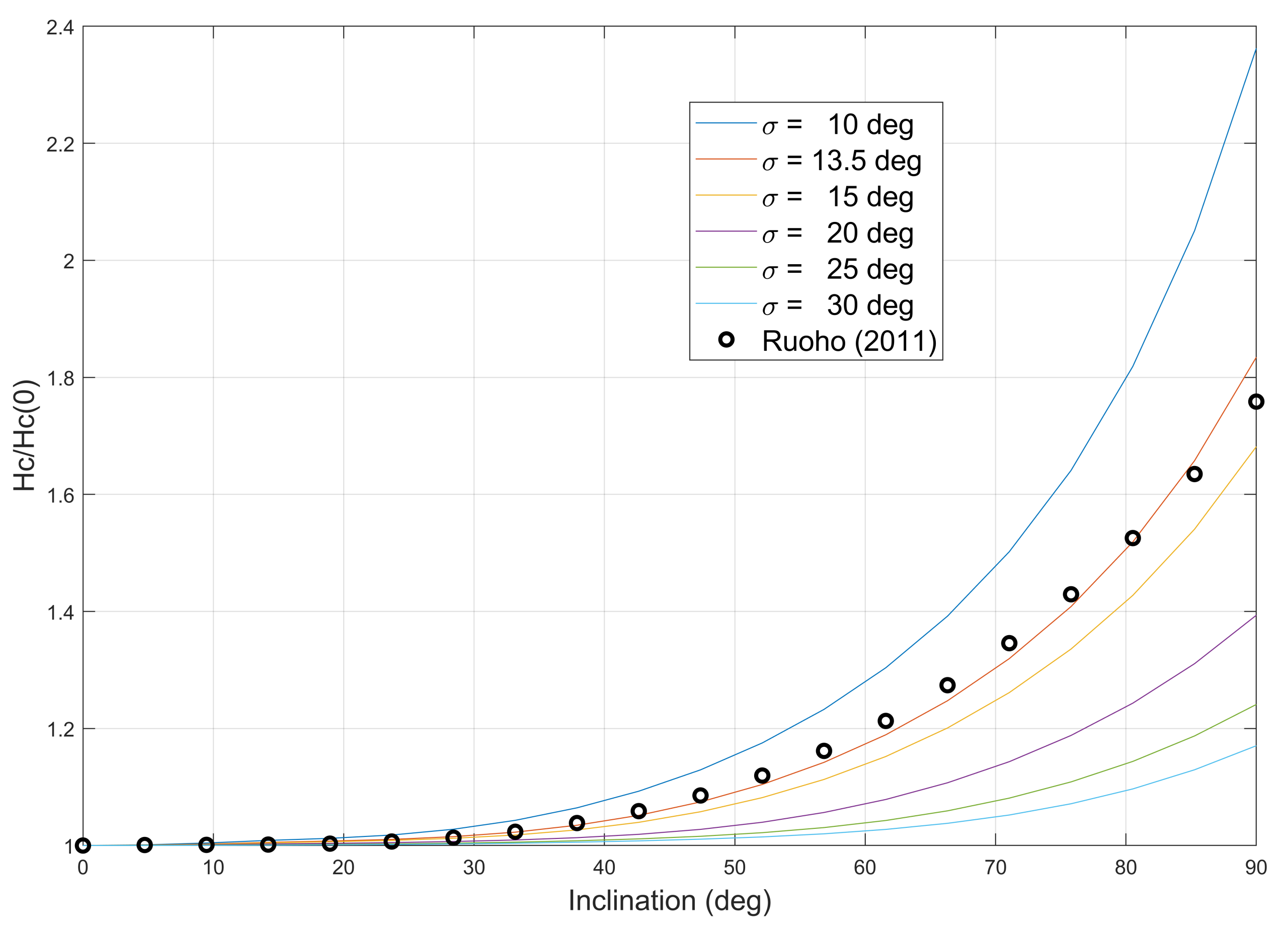
From our original point of view of ferrites, an important caveat-these results were for Neodymium magnets. Whether or not ferrites exhibit a similar relationship is the big question.

---

Check out EMDtool - Electric Motor Design toolbox for Matlab.

Need help with electric motor design or design software? Let's get in touch - satisfaction guaranteed!

Tesla Cybercab Motor – Demagnetization Point-of-View