Stop Playing with Hysteresis - pt. 2

In the previous part, we got to know the play hysteron and its cousin the stop hysteron. Today, we’ll take a deeper look on how they behave as a group, and where they can be taken from the simple case.

Behaviour

To recap, a play hysteron can be understood as an inertial less spring-friction system, with a spring coefficient $k$ and a constant friction force $r$ . This, as long as the input $\mathbf{B}$ remains small enough, the hysteron state $\mathbf{m}$ (and the output of the play hysteron) does not move:

$|\mathbf{B}-\mathbf{m}| \leq \frac{r}{k}.$

And, once we do move, all work that we put into the system gets dissipated as friction heat

$\mathbf{H} \text{d} \mathbf{B} = r\text{d}\mathbf{m},$

where $\mathbf{H}$ is now the spring force $k\left(\mathbf{B}-\mathbf{m}\right)$ , also known as the output of the stop hysteron.

Importantly, from these two things alone we get the loss behaviour for both the alternating and rotating case.

Alternating losses

As we have seen, when the hysteron is moving, it lags the input by the amount $\frac{r}{k}$ . Thus, say we have an uniaxial alternating magnetic flux density with the amplitude of $B_1$ . For simplicity, assume we have no DC component, even though we know now that it does exactly zip-all to the losses. Then, at the reversal point, the hysteron lies at

$m_1 = B_1 - \frac{r}{k}.$

Now, this assumes that $m_1$ is positive. If it’s not, then the excitation is too weak to move the hysteron – we only wiggle the spring part and move energy into it and than then back again, with no dissipation.

That said, if we do move, then our peak-to-peak amplitude is

$\Delta m = 2(B_1 - \frac{r}{k}),$

and the net energy dissipated per cycle

$E = r \Delta m = 4 r (B_1 - \frac{r}{k})$

as we do the peak-to-peak traversal twice – from minimum to maximum and then back to minimum again.

Now, this is just the loss per a single unweighted hysteron – in practice we have an ensemble of $M$ hysterons with associated weights. This is programmatically perfect, but what little I remember of finite sums evades me right now, so let’s look at the limit case of infinitely many hysterons and a continuous distribution of weights.

We get for the ensemble losses

$E = \int\limits_{0}^{r} w(\hat{r}) 4 \hat{r} (B_1 - \frac{\hat{r} }{k}) \text{d}\hat{r} .$

For the typical case of a constant spring constant $k=1$ for all hysterons, we get $r=B_1$ for the upper limit.

Now, we obviously still have the unknown weight function, which ultimate depends on how we want the losses to grow with $B_1$ . But, for the simplest textbook-like case, we can set

$w(r) = \frac{1}{r}$

(and conveniently ignore the singularity), in which case we get

$E(B_1) = 4\int\limits_{0}^{B_1} B_1 - \hat{r} \text{d}\hat{r}=2 B_1^2.$

In other words, we get the Bertotti-like quadratic dependency – ta-dah!

In the slightly more general case with a non-unity $k$ , we get $r = kB_1$ for the upper limit, and

$E(B_1) = 2 k B_1^2$

for the total losses. Meaning, even though the losses per a single hysteron are only weakly dependent of the stiffness, it does influence how many hysterons active (aka slide) for a given input, and thus the ensemble-level losses.

Rotational losses

Now, let’s consider instead the rotational case, again with a given amplitude $|\mathbf{B}| = B_1$ . Now, although this may not be immediately obvious, in the steady state we have $\mathbf{m}$ and $\mathbf{B}-\mathbf{m}$ perpendicular to each other. Thus, we can solve for the amplitude

$m:=|\mathbf{m}| = \sqrt{ |\mathbf{B}| - |\mathbf{B}-\mathbf{m}|^2 } = \sqrt{ B_1^2 -(r/k)^2 }.$

Here, the last expression has been simplified by realizing that the hysteron spends the entire time sliding, so it lags $\mathbf{B}$ by $r/k$ .

Now, we get the energy dissipated during an entire cycle from the net distance slid times the friction force

$E=2\pi m \cdot r = 2\pi r \sqrt{B_1^2 -(r/k)^2 } .$

Less-simple mathematics

Now, a little bit of more advanced mathematics. They are not really needed for the simple hysterons, but they can be handy when analysing whatever smart extension you might have in mind.

Somewhat unsurprisingly, we can introduce a couple of potentials to help us out. Because who doesn’t like potentials? Life wouldn’t have meaning without a potential or too.

Sigh. Here goes.

First, we have the kinetic energy of the spring

$E(\mathbf{B}, \mathbf{m}) = \frac{1}{2} \left(\mathbf{B} - \mathbf{m}^\text{T} \right) k \left(\mathbf{B} - \mathbf{m} \right).$

From this alone, we get the forces acting on the internal state $\mathbf{m}$ and the output force as

$\mathbf{H} = \frac{E}{\partial \mathbf{B}}=k(\mathbf{B} - \mathbf{m})$

$\mathbf{F} = \frac{E}{\partial \mathbf{m}}=-k(\mathbf{B} - \mathbf{m})$

In addition, we can define something called a dissipation potential – in our case so far:

$\chi = r |\Delta m| .$

Finally, we get the update rule for the internal state $\mathbf{m}_{k+1}$ as

$\mathbf{m}_{k+1} = \text{argmin}_{ \mathbf{m}_{k+1}} E(\mathbf{B}, \mathbf{m}_{k+1}) + \chi(\mathbf{m}_{k+1}, \mathbf{m}_k) .$

Assuming the potential function is convex (i.e. the Hessian matrix of $E$ is positive-definite) we get an unique minimizer by setting the gradient to zero

$\frac{\partial}{\partial \mathbf{m}}( E + \chi) = 0.$

In the simplest case, what we have been discussing so far, we can easily see in 1D that the update we get – assuming that we do the update and don’t stay stationary – from minimizing the potential is

$m_{k+1} = B_{k+1}-\frac{r}{k} \text{sign}(m_{k+1}-m_{k}).$

The same applies for 2D (or 3D for that matter); we just have to replace the sign by the unit vector $\mathbf{\Delta m}} / |\mathbf{\Delta m}} |$ where the Delta-m is the difference between the previous and current values. In other words, we have a unit vector pointing into the direction where $\mathbf{m}$ moves. Please now note that the update rule is already nastily nonlinear, technically speaking – the sign function / calculation of the unit vector is not a linear operation. However, in this simple case we can see with our third eye that movement vector is parallel to $\mathbf{B}_{k+1}-\mathbf{m}_k$ .

While this potential-thing absolutely sucks in almost every respect, it does give us a nice-ish theoretical framework that we can then later violate on purpose rather than by accident. The nice thing about the potential framework is that as long as we respect it, we can guarantee that we don’t accidentally inject energy into the system out of thin air, or make it disappear without us noticing. Specifically, we know that the energy coming from the magnetics $\mathbf{H} \text{d} \mathbf{B}$ equals the energy going into the elastic potential plus the energy dissipated.

How to make everything suck

Anisotropy

From how I wrote the potential, an obvious generalization is an anisotropic spring:

$E(\mathbf{B}, \mathbf{m}) = \frac{1}{2} \left(\mathbf{B} - \mathbf{m}^\text{T} \right) \mathbf{K} \left(\mathbf{B} - \mathbf{m} \right)$

with some nice stiffness matrix $\mathbf{K}$ . It might be nice for stuff like modelling anisotropy, or, used together with some other approaches in modelling the rise and fall of rotational losses with $B_1$ .

Sadly, an anisotropic spring alone is enough to make life suck again, since our distance-to-yield condition is now an ellipse

$|\mathbf{K}(\mathbf{B}-\mathbf{m})| \leq \frac{r}{k},$

making the position-update step nontrivial. Furthermore, the update direction isn’t generally parallel to $\mathbf{B}_{k+1}-\mathbf{m}_k$ any more, giving us extra nonlinearity.

While we might derive an analytical solution for small-enough steps, we would also have to prove that we always get a meaningful update even when steps are no longer small, and then implement some downhill sled-ride gradient descent as a fallback option, and then make sure all those work fast enough for 100k elements with 5-10 Newton steps each multiplied with a few dozens or low hundreds of time-steps…things get difficult fast.

Prodding at r or k

Or, we might like to have either $r$ or $k$ depend on something – either $\mathbf{B}$ or $\mathbf{m}$ most likely, in order to attack any of the shortcomings of the hysteron model for magnetics. The DC-bias insensitivity or the less-than-realistic dependence of rotational losses on $B_1$ for instance.

Modifying $k$ is somewhat nasty. If we let it depend on $\mathbf{m}$ , we very easily lose the convexity of the potential. Meaning, we can’t guarantee that the derivative-equals-zero update scheme yields us the true minimum. In fact, if you absolutely want to guarantee the convexity of the overall potential, while maintaining the quadratic-in-displacement spring potential, you get some very nasty and restrictive conditions on $k'$ and $k''$ .

On the other hand, if you tie $k$ to $\mathbf{B}$ , you directly start introducing wonkiness into the output $\mathb{H}$ – remember that we have

$\mathbf{H} = \frac{E}{\partial \mathbf{B}}.$

This only has an effect on the elastic part, when the hysteron isn’t yet sliding.

Modifying $r$ is comparatively simpler, is it doesn’t influence the convexity conditions or the output, other than changing the sliding threshold $|\mathbf{H}| = r$ .

Naturally, we could also approach this problem by having the elastic potential itself be an arbitrary function, rather than insisting it be product of a spring coefficient and a distance term. But, the same limitations as before still apply.

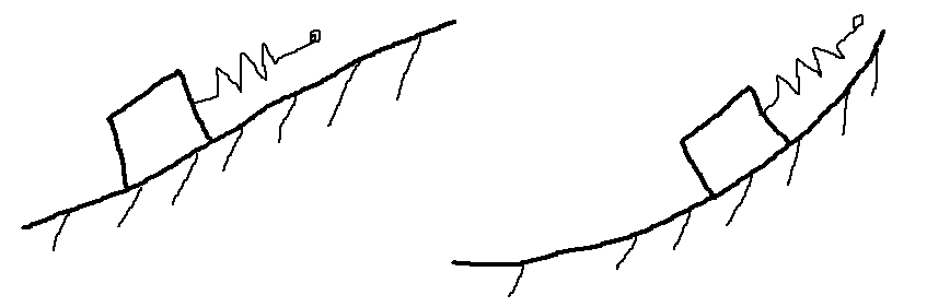
Potential landscape

Finally, we could introduce an additional potential, to be summed with the elastic potential and not depending on the distance between $\mathbf{B}$ and $\mathbf{m}$ .

For instance, we could have

$\Phi (\mathbf{m}) = \text{atanh}\left( \frac{|\mathbf{m}|}{m_\text{sat}} \right) .$

This potential would explode towards infinity as $\mathbf{m}$ approaches a given saturation threshold $m_\text{sat}$ .

Even with less extreme values, the slope of the landscape potential influences how much the hysteron moves, and how much energy is therefore dissipated. This can again be seen from the 1D example. With the same minimization approach as before, we get the condition

$-k(B-m_{k+1}) + \partial_m \Phi(m_{k+1}) \pm r = 0.$

By linearizing the landscape potential around the previous step

$\partial_m \Phi (m_{k+1}) \approx \partial_m \Phi (m_k) + \partial_{mm} \Phi (m_k) \cdot (m_{k+1}-m_{k})$

and reorganizing, we get

$m_{k+1}\left(k+\partial_{mm} \Phi \left(m_k\right)\right) = kB - \partial_m \Phi (m_k) - \partial_{mm} \Phi \left(m_k\right) m_k \mp r.$

In other words, a landscape with a constant slope (be it uphill or downhill) is seen as a simple bias force on the right side. It if curves, i.e. if the slope gets steeper (or flatter) as you move, it also influences the step size via the $1 /(k+\partial_{mm} \Phi)$ term.

Check out EMDtool - Electric Motor Design toolbox for Matlab.

Need help with electric motor design or design software? Let's get in touch - satisfaction guaranteed!

Stop Playing with Hysteresis – pt. 2

Antti Lehikoinen