On Eddy-Current Iron Losses | Antti Lehikoinen

Preface

I had already written this post up to the analytical methods section when WordPress saw fit to lose all my progress for some reason. So, if you get an aura of pissed-offness from the first few sections, it’s not you. It’s not me either, it’s TurdPress.

Introduction

Ah, the iron losses. Nobody knows to how to actually compute them. Even if you had a perfect material model (which you don’t), things depend so much on the actual manufacturing process (and e.g. the current condition of the tooling used, subject to changing over time).

Sure, you can slap on a build factor based on measurement data, or even adjust a fancy model based on it if you have one, but doing that all a priori takes a quite a lot of experience, or an Ouija board.

That said, there are some things you should now, or at least wouldn’t be worse off knowing. Moving into the know-what-you-don’t-know territory, in other words.

Read on to dive into a specific part of iron losses.

A brief history

Disclaimer: I’ve never done a proper literature review on the history of iron losses. So, I’m bound to get some historical details at least slightly wrong. If you do actually know better, please let us know in the comments – I’ll edit the text accordingly with full credits to you should you wish.

Now, the way I see it, iron losses in electrical steel sheets happen on multiple levels, or physical scales. There’s stuff going on on the grain or domain or whatever level. Then there’s the level of eddies within the laminations – the topic of this post once we get that far. Finally, there’s bound to be the short-circuit or two between the laminations, leading to eddies flowing over multiple laminations (interlaminar is the magic word for Google).

This is also reflected in the classical division of iron losses into hysteresis and classical eddy-current losses.

Hysteresis losses are, more or less, thought to be related to magnetic domain wall motion, pinning in defects, microscale eddies circulating next to the moving domain wall motion. What I don’t know is if the microscale eddies are the only method of energy dissipation, or if there’s some lossy chemical-physical thing going on with the pinning in addition. If you know, let me know.

Then there are the so-called classical eddies, i.e. eddy-currents circulating within a single lamination, governed by the classical Maxwell’s equations.

Finally, many people include the third loss component – the so-called excess losses. To my best knowledge, the jury’s still out on whether these losses actually exist, or if the apparent frequency-and-flux-density dependence is explained by the uneven distribution of the flux density across the depth of the lamination, caused by the classical eddies.

Which, coincidentally, brings us to the actual topic today.

‘Classical’ eddies

So, what actually happens inside an electrical steel, when subjected to time-varying flux density on the plane of the lamination.

Eddies are induced in it, obviously, steel being conductive and all.

These eddies cause losses – hence the ‘eddy-current’ term in the classical loss division.

Additionally, they oppose the change in the flux density, although this effect is often ignored in analysis. In other words, the B-versus- is assumed to follow the single-valued BH-curve. At least, this is the case in motor design – magnetic components people may be more advanced in this respect.

Simple approaches

The simplest way to analyze the eddies and eddy losses is by assuming they don’t influence the flux density. More precisely put, the flux density is assumed to be uniformly distributed across the thickness of the lamination (let’s call it the z-coordinate here). Finally, by assuming that the variation of the flux density along the plane of the lamination (x- and y-dependency) is weak compared to what happens in the z-direction, we see, with our third eye, from the Lenz law

$\nabla \times \mathbf{E} = -\frac{\text{d}}{\text{d}t}\mathbf{B}$

that the current density (amplitude) inside a single lamination is

$J(z) = z \sigma \frac{\text{d}}{\text{d}t}B(t)$

where B(t) is the amplitude of the time-varying flux density – remember that we don’t care about the xy-dependency per our assumptions. Note that our z-coordinate is now centered at z=0, so that the net induced current averages to zero.

Integrating this over the lamination thickness d, and then dividing by said d to get the volumetric loss density yields

$\int_{-d/2}^{d/2} \frac{J^2(z)}{\sigma} \text{d}z = \frac{\sigma d^2}{12} B^2(t)$

With this reasoning, the simplest way to actually include the damping effect from the eddies into an electromagnetic simulation is to modify the (rate-independent) BH-behaviour into

$\mathbf{H}(\mathbf{B},t)=\mathbf{H}_{\text{static}}(\mathbf{B})+\frac{\sigma d^2}{12}\frac{\text{d}\mathbf{B}}{\text{d}t}$

Finally, assuming a sinusoidally-varying flux density and computing the time-average yields us the probably-familiar analytical eddy-current loss density term

$\langle P \rangle=\frac{\sigma \pi^2 d^2}{6} \times f^2B^2.$

Not-so-simple any more

Now, reality is often ~~disappointing~~ more complex than simple theory predicts (you can also interpret that as a comment on the online dating advice, or pretty much any advice online, as per my previous post). And one way in which things do get more complex is via the effect of the induced eddies on the flux density.

When (re-)deriving the simple analytical expressions above, we assumed the flux density to be independent of the z-coordinate. In other words, we assumed it to be uniformly distributed along the thickness of the lamination.

This, in reality, is not the case. Eddy-currents appear to prevent the flux from penetrating into a conducting body (or rather, prevent the change in flux, but for periodically-varying flux density, the end result is pretty much the same), and they always succeed to some degree. There are no perfect insulators, after all.

Practical example

In steel laminations, when considering the typical sheet thickness-vs-frequency pairs, the effect is often quite noticeable, indeed. Let’s look at an example.

The animation below shows two rather typical examples: an 0.2 mm lamination with 1 kHz sinusoidal excitation, and an 0.5 mm lamination at 50 Hz. In both cases, the average flux density (zero-to-peak) is 1.5 T. The two curves show how the flux density varies across the thickness (the symbol d) of the lamination.

As can be seen, the skin effect drives the flux density towards the – *drumroll* – well, skin. Aka, the surface of the lamination. The effect is obviously more pronounced in the 0.2 mm 1 kHz case, but even the 50 Hz case does have some noticeable variation.

Practical effects

So, what does this mean in practice?

For one, it influences the magnetic field required to drive the flux density. Earlier, we ‘derived’ (as in I copy-pasted it from folks who know better) the

$\mathbf{H}_{\text{static}}(\mathbf{B})+\frac{\sigma d^2}{12}\frac{\text{d}\mathbf{B}}{\text{d}t}$

as an approximation of the eddy-current-related damping.

In reality, there are obviously more complex dynamics at play, with the history of the flux density also influencing the required field right now.

The following figures should illustrate this. They demonstrate the BH-loops of an 0.2 mm steel, with the average flux density alternating sinusoidally (at a few different amplitudes in each pic) at 1 kHz, 5 kHz, 10 kHz, and finally at 30 kHz. Shown are the case without skin effect (i.e. with just the $\frac{\text{d}\mathbf{B}}{\text{d}t}$ correction), and with skin effect, i.e. with the distribution of the flux density inside the lamination actually modelled.

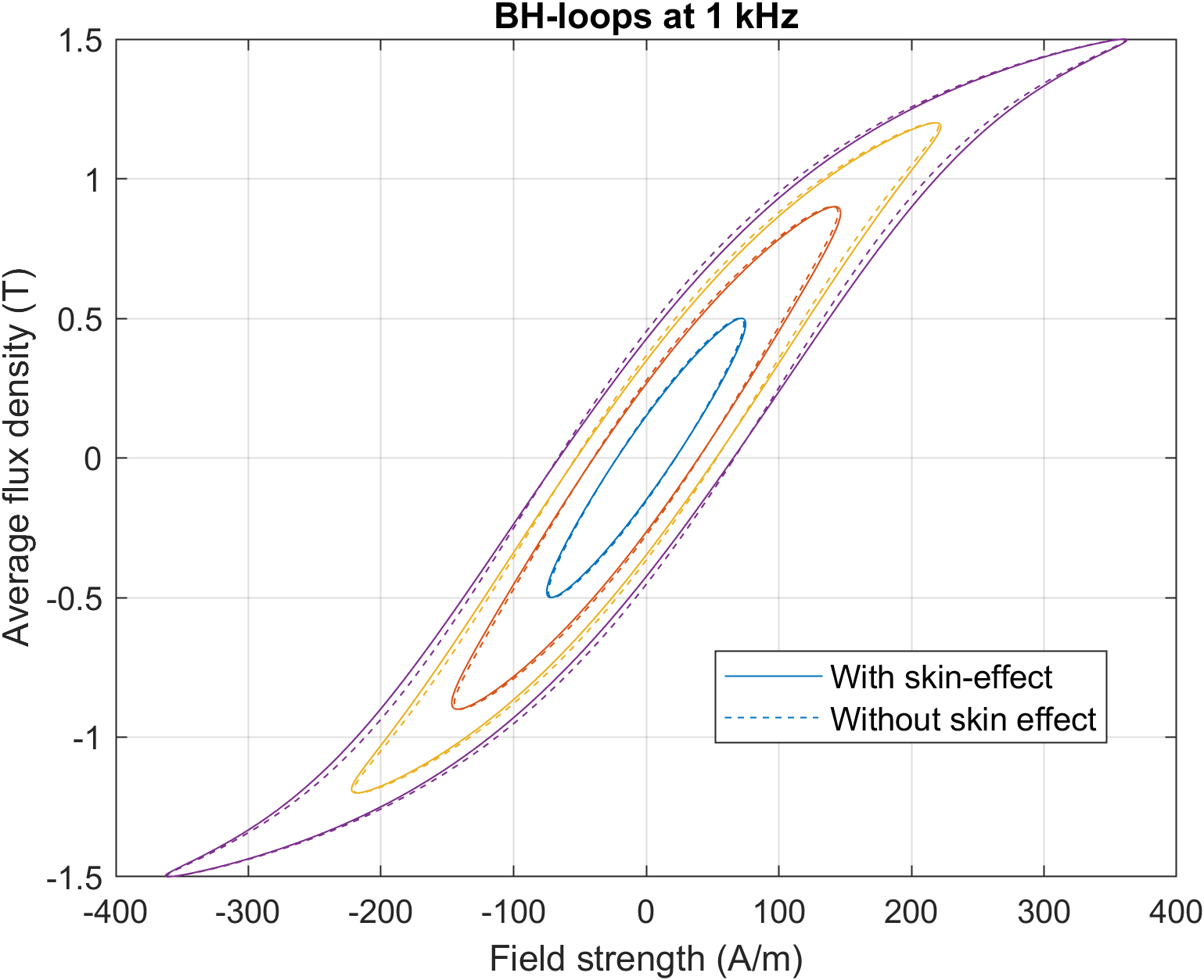
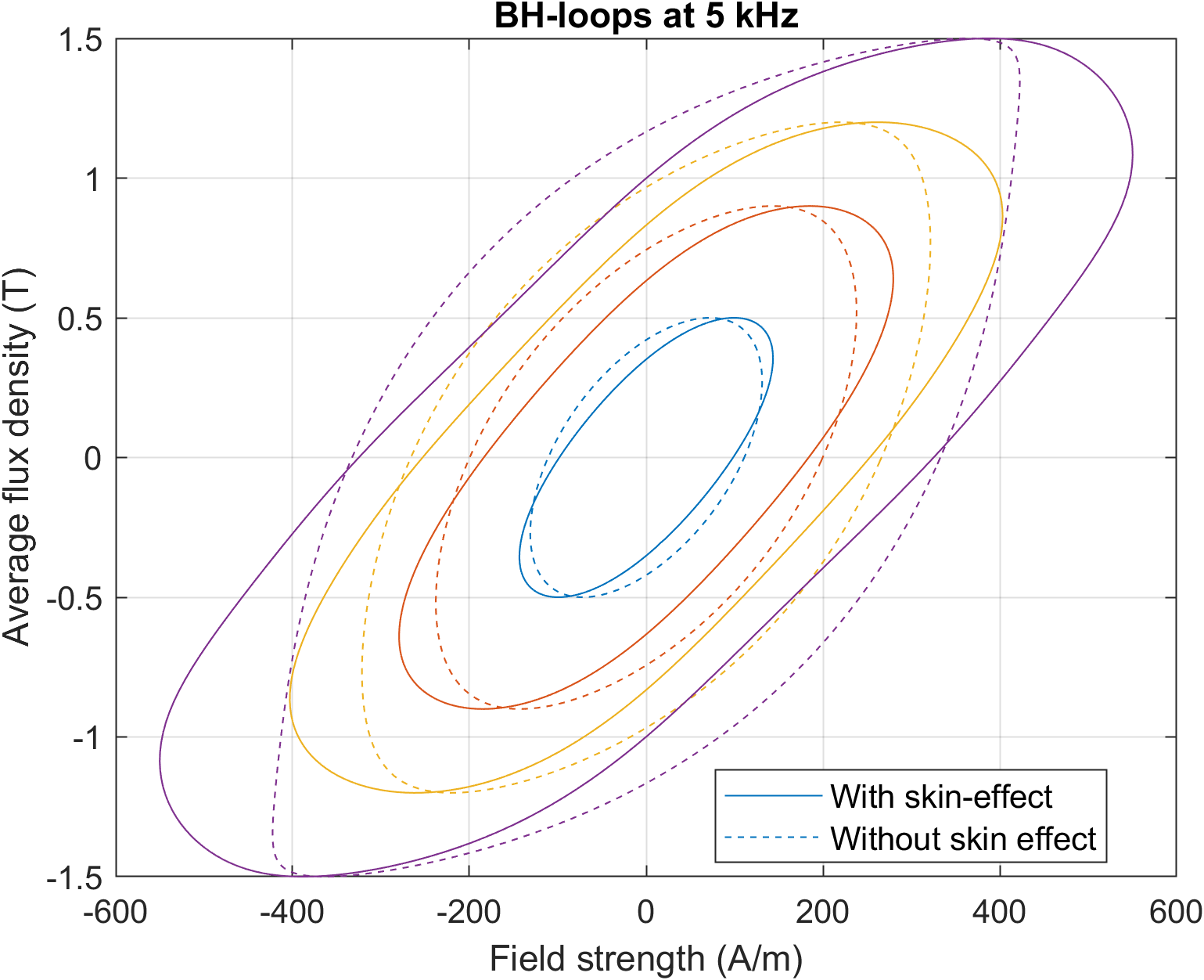
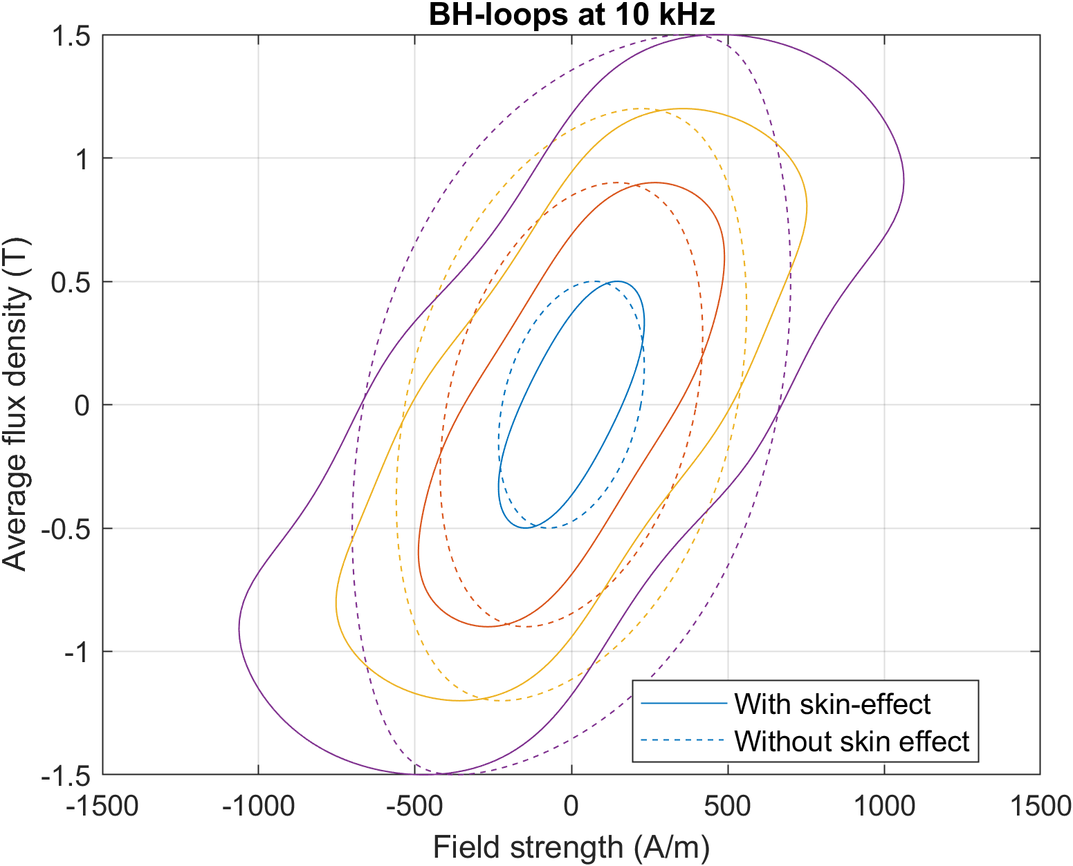
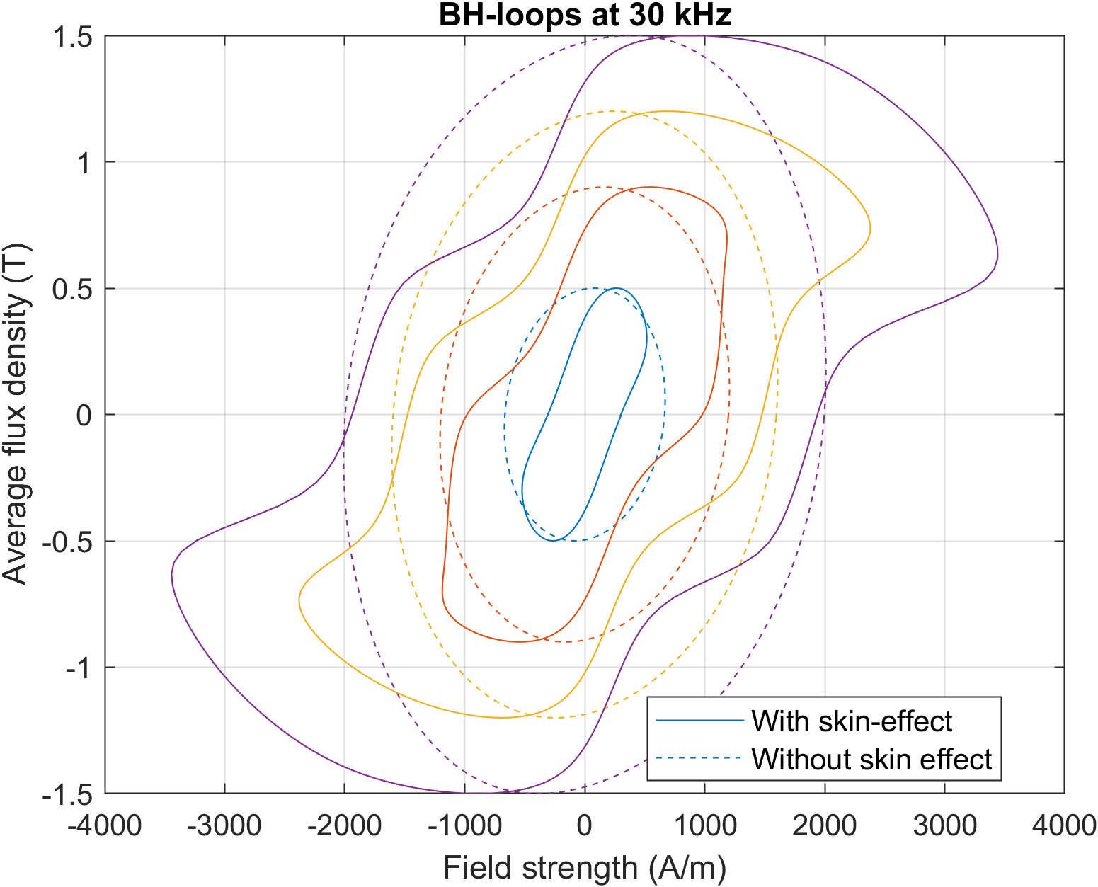
As can be seen, at 1 kHz both approaches yield rather similar results. However, as the frequency increases and the skin depth becomes significantly smaller than the lamination thickness, the two approaches start to diverge more and more.

At very high frequencies, things become downright wonky – which brings us to our next topic.

How to model

When it comes to the theory, this phenomenon is easy to model with 3D Maxwell’s equations. Granted, you need a hysteresis model for the (assumed) static hysteresis $\mathbf{H}_{\text{static}}(\mathbf{B})$ which nobody can do, but otherwise things are simple.

Obviously, this approach is a computational nightmare, requiring an extremely dense mesh (compared to the other dimensions of a motor or generator) to cover the depth of the lamination.

One approach to circumvent this problem was (to my knowledge) first proposed by Gyselinck (IEEE Xplore here, preprint here). We begin by taking the Ampere’s law

$\nabla \times \mathbf{H} = \mathbf{J},$

writing the electric field with the material equation $\mathbf{E} = \mathbf{J} / \sigma$ , plugging things into the Lenz law

$\nabla \times \mathbf{E} = - \frac{\text{d}\mathbf{B}}{\text{d}t}$

to get

$\nabla \times \nabla \times \mathbf{H} = - \sigma \frac{\text{d}\mathbf{B}}{\text{d}t}.$

Finally, the curls are written open and the partial derivatives with respect to x and y are neglected (under the assumption that the other dimensions are much larger than the lamination thickness, and the variations of B are correspondingly slower in-plane) to get a 1D diffusion equation

$\frac{\partial^2\mathbf{H}(z)}{\partial z^2} = - \sigma \frac{\text{d}\mathbf{B}(z)}{\text{d}t},$

where the vectors are now assumed to lie on the xy-plane with no change in notation due to laziness.

Gyselinck’s approach was to write B as a spectral expansion

$\mathbf{B}(z) = \sum_{i=0}^N a_k \alpha_i(z),$

i.e. as a sum of known polynomials weighted by unknown coefficients a to be solved. We all agree here.

Now, my gut feeling would have been to solve the diffusion equation with the finite element (or spectral) approach, while keeping the exact $\mathbf{H}(z)=\mathbf{H}_{\text{static}}(\mathbf{B}(z))$ relationship from the material model, whether hysteretic or not.

In retrospect, this would have been tricky, thanks to the double derivative there – no easy way to get rid of it. Indeed, Gyselinck’s really smart twist was then to write H in such a way that the diffusion equation is satisfied exactly, by utilizing the second antiderivatives of the basis functions used for B, plus an extra constant term.

As this approach does not generally satisfy the material equation in an exact fashion, we now require it is satisfied in the so-called weak sense, aka FEA-style,

$\int_{-d/2}^{d/2} \alpha_i(z) \left(\mathbf{H}(z) - \mathbf{H}_{\text{static}}(\mathbf{B}(z)) \right) \text{d}z = 0$

for all values of i.

Issues and limitations

Take a look at the high-frequency BH loops. You can see how they start to slightly resemble a flower or something like that. I haven’t studied this very phenomenon in much detail, but there are multiple factors that might be contributing to this.

The first is the plain old implementation error by yours truly. I have double- and triple-checked everything, but it’s still possible. I give it a 20 % chance.

The second is pure physics. As seen from the animation, the eddy currents drive the flux density towards the surfaces of the lamination. Now, when the edge flux density hits saturation, you can intuitively expect some kind in the field strength needed to drive it. Likewise, the flux in the center parts is lagging the surface value, which also brings some dynamics to play.

The third might be limitation in the model itself, namely in the choice to use a polynomial basis for modelling the flux density across the entire depth of the lamination.

Indeed, the animation below shows the modelled flux density distribution inside an 0.2 mm lamination, at 30 kHz alternating flux density with a whopping 1.7 T average amplitude. Quite a violent excitation, yes, but it does illustrate the phenomena.

Now, what you could pretty much expect to happen, and what is somewhat supported by the simulated distribution too, is that the flux density on the surface reaches saturation first (duh). Then, it more or less stays there, while the rest of the lamination progressively catches up. Indeed, at many instants of time, you could expect almost a piecewise-continuous pattern: a constant at-saturation part near the surfaces, with a smooth dip in the middle.

However, what you also see are same oscillations or ripples that you really wouldn’t expect to be there, for any physical reason. I suspect these are some out-of-wedlock child of the Gibbs phenomenon – the polynomial basis used is simply unable to represent the desired flux density distribution too well.

In any case, I will have to try to find the time to double-check this with the plain old vector potential represented with FEA hat functions – they work just as fine in one dimension too.

Conclusion

You have now read some ramblings about lamination-level eddy-current losses – the so-called classical eddies in other words.

Check out EMDtool - Electric Motor Design toolbox for Matlab.

Need help with electric motor design or design software? Let's get in touch - satisfaction guaranteed!

On Eddy-Current Iron Losses