Stop Playing with Hysteresis | Antti Lehikoinen

Summary

As the title suggests, with wordplay downright hysterical (thanks, Robert, for the extra pun!), this post is an informal-ish introduction to the play and stop hysterons. As we’re speaking about motors here, the focus will be on modeling ferromagnetic hysteresis, primarily in electrical steel and the like. We’ll cover why hysteresis is kinda important in the first place, how the play and stop look in their simplest form, and where we can take them from there.

Let’s dive in.

Hysteresis – what and why?

Let’s begin with hysteresis itself. As you hopefully know, electrical machines have this nice little feature called iron losses – put a flux density in that changes in any way, and losses come out. The magnetic flux density B does not nicely follow the field strength H, but lags behind in one way or the other, depending both on how and how fast H is changing. In one dimension, we get the well-known loop in the BH-plane, the loop area representing the energy loss per each cycle. Reality hates us, however, and things are multidimensional, so that simplistic idea doesn’t get us too far.

I’ve already written a post on eddy-current losses. You can argue ad infinitum on if and how you can or should split the losses and if excess losses actually exist or not for that matter, but how I split them here is as follows. Eddy-current losses are what you get from the macroscopic Maxwell equations (insert Maxwell the cat here), mainly the Lenz law for the eddy-currents and Ampere’s law on how said eddies influence the flux density.

Hysteresis, on the other hand, I define here as the lossy and (duh) hysteretic BH-behavior you get at very low rates of change, where the contribution of the eddy currents tends to zero. Rate-independent hysteresis, in other words. Incorrect words, most likely, in some particular flavor or nuance. I am not an expert on this.

So, the behavior that is fundamentally iron, unperturbed by mortal concerns like time or conductivity.

One might think that hysteresis modeling, and hysteresis losses in particular, would be becoming less and less relevant with the continuing push towards higher frequencies (I do lots of work on high-speed machines, so please send your monies my way now). One would be wrong.

True, frequencies are increasing across the (dash)board. As eddy losses grow somewhat like with the frequency squared, and hysteresis only linearly with the frequency (not because they care about the frequency as per my definition – they only care about change, but a higher frequency means you can fit more of said changes in any given period of time, usually a second for a sane person), they do tend to become more significant at higher frequencies.

However, at the same time, the average sheet or lamination thickness has steadily decreased. As eddies also care about the thickness squared, their relative share of the total losses has remained roughly the same. There’s also probably something in thin sheets that makes them particularly hysteretic, but again – not my particular expertise.

So hysteresis is important.

Sadly, hysteresis is also a colossal pain to model.

Let’s play

With the pre-ramble out of the way, let’s jump straight into play hysterons. Imagine you have a cup or a glass on the table, and you have a straw or perhaps a pencil inside the cup. Now, please move the cup with the tip of the straw, without taking it out of the cup (and without tipping the cup or spilling your morning coffee/tea/whisky).

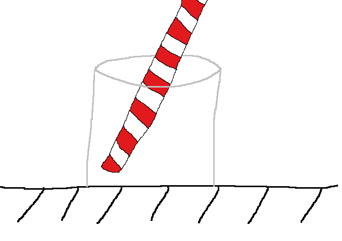
No LMM was harmed in the making of this image.

That’s a simple play hysteron, in a confusing nutshell.

The coordinates of the tip of the straw – on the xy-plane that is your table – are your input. The coordinates of the mug (its center of gravity, again in xy-terms only) are your output.

What makes this example a hysteron is the fact that the cup is larger than the straw, meaning you can wiggle the latter around quite a bit without the former moving. The cup only shifts when you push the straw against the wall. The output is lagging the input, in other words.

Also, wiggling the straw inside the cup is lossless. Roughly so in reality, perfectly so in the realm of our example. Only when the mug itself moves are you spending – dissipating – energy in moving the cup against the will of friction.

Another example

Granted, there is another example that is perhaps more commonly used to illustrate the play hysteron – if it is illustrated at all via anything other than update equations. I find it a tad harder to imagine, so hence we went through the mug-and-straw thing first. But, the second example is a little more mathematics-friendly and extendable, so let’s also do it.

Imagine we still have our table, and an object lying on it. We have a spring connected to the object, its other end connected to our finger (in a non-destructive fashion, I hope) or whatever we want our input to be. Again, the coordinates of the object will be our output.

Now, we want some kind of friction between the object and the table, again. All good so far.

Where things get a little unintuitive for anyone with a little knowledge of basic physics are the following two assumptions.

First, we want the same amount of friction regardless of if the object is moving or stationary. Equal static and kinetic friction, in other words.

Also, we want the object to be massless, or close enough to massless so that its motion is governed by the friction and spring forces alone, Newton’s second law be damned.

With these assumptions now hopefully internalized, we get the same behavior as before, only with some math to describe it now.

If we keep our finger close to the object, and the spring rather relaxed, we only exert a little force on it. Less force than the friction does (or rather, the friction exerts exactly as much force as is needed to keep the object stationary), so the object stays put. We can wiggle the finger a little, just like the straw inside the mug.

Now, if we try to pull our finger away, we meet a point where the string force overcomes the friction. Since the object is assumed inertialess, it will instantly start moving exactly at the same velocity as our finger, following it around at such a distance that the spring force exactly matches the friction. That is as long as we keep moving roughly in the same direction – if we do a reversal, the spring again slackens and the object stops.

Stop

The spring-and-friction force example is, in my opinion, slightly more suitable than the mug-and-straw version for introducing the cousing of the play – namely the stop hysteron. The mathematical term might be a ‘dual,’ though that is yet again one language I’m not fluent enough to be certain.

Anyways, the output of the stop hysteron is the spring force.

That’s it. Or, if you insist on the mug-and-straw example, it’s the distance between the straw and the mug center. Though, I must caution you that this definition sadly gets very muddy once we move into the generalizations later.

Now, many authors like to define the stop hysteron – or its update rules – independently of the play. That is definitely an option; however, I find said rules extremely confusing, while the spring-force definition can be explained with, umm, a spring. And a force.

Magnetics

In (ferro)magnetics, the play and stop hysterons lend themselves naturally to direct and inverse modeling of the BH-behavior.

The output of the play hysteron lags the input, so a natural way of organizing things would be to have the magnetic field H as the input, and either the flux density B or the magnetization / magnetic polarization as the output.

Now, you could argue intensely on whether the output of the stop hysteron actually leads the input, or if some other term would be correct. We can all probably agree that what it does not do is lag the input, so hence the natural order of things here is the opposite. We have H as the output, and flux density B as the input.

Simple mathematics

I’ve postponed it this far, but some mathematics are needed. Sorry. Some readers will think I should have introduced maths earlier, so sorry for that, too. Here goes.

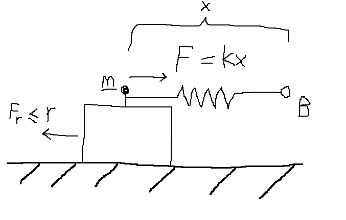
Let’s denote the internal state – position – of the hysteron as m. Then we have for the spring force

$\mathbf{F} = k(\mathbf{B}-\mathbf{m}),$

where k is the spring constant.

At the same time, we have the friction force – denote it r.

Now, our hysteron stays stationary whenever $|\mathbf{F}| < r$ . If the force tries to get too large, the hysteron slides so that we have exactly $|\mathbf{F}| = r$ . Again, remember that we have no inertia here, so the spring force never gets strictly larger than the friction.

Expressed in a more mathematical way, and again reflecting the role of mechanical engineering in the models that we so like, we say that we have yield limit

$|\mathbf{B}-\mathbf{m}| <= \frac{r}{k}.$

Anytime we wiggle the input within the limit, the hysteron stays put. We can put energy into the spring by pulling it tighter, but we recover it all if we let it relax again.

By contrast, if we end up moving the hysteron, we permanently lose some energy in the friction. Here, the energy equals the force times distance-moved rule, or expressed differentially

$dE = r|d\mathbf{m}|.$

Practical usage

The behaviour of our single hysteron is piecewise-linear. This is alone is rather insufficient for most purposes, so in practice, an ensemble of multiple hysterons is used.

Commonly, the spring constant k is fixed to a constant value, and a range of friction forces r or thresholds is used. Finally, a weight w is assigned to each hysteron.

$\mathbf{H} = \sum\limits_{k=1}^M k w_k \left( \mathbf{B}-\mathbf{m}_k\right).$

The state $\mathbf{m}_k$ is then updated based on the principles earlier.

Now, there are a few more details worth noting.

First, many authors omit the spring constant k. I don’t like this. It fuzzies the physics of the behaviour, and introduces a unit mismatch, requiring as to hide the units in the weights which very much goes against how the concept of weight is commonly understood in mathematics.

Secondly, shape functions are often used. Meaning, we don’t use the outputs of the hysterons as such, but first shape them by non-hysteretic functions f:

$\mathbf{H} = \sum\limits_{k=1}^Mw_k f_k \left( k\left( \mathbf{B}-\mathbf{m}_k \right)\right).$

Shape functions can and will make the non-dissipative part of the behaviour into whatever we want it to be. Meaning, when $\mathbf{m}_k$ is stationary, we can turn the linear slope $k\left( \mathbf{B}-\mathbf{m}_k \right)$ into whatever we wish – usually either saturation or a sharp increase.

Pros and Cons

Hysteron models have many attractive properties. They are (at least in the form presented here) natively vectorial, meaning they play nicely with rotating machines.

They work well with finite element analysis, too. The output is continuous, even if it isn’t smooth everywhere. A B-to-H version (the stop hysteron, or using the ‘spring force’ as the output) exists, meaning the model can be plugged into a typical FEA package as such, without requiring an inner iterative solution. The evaluation of the model is simple, too – a single-pass linear operation with no iterations needed.

Finally, a very nice property for post-processing: we get an instantaneous loss density from the hysteron movement and friction force, right away. Granted, we have a settling period depending on the initial conditions for $\mathbf{m}_k(t=0)$ . For instance, setting $\mathbf{m}_k(t=0)=\mathbf{B}(t=0)$ requires $\mathbf{B}$ to move enough for all hysterons to become active, yielding smaller losses initially compared to the steady-state behaviour. But still, we do get the losses directly, without having the integrate $\int \mathbf{H} \cdot \text{d}\mathbf{B}$ and trying to estimate how much of the result is actually lost for good, how much is energy in the magnetic field that might yet be regained, and how much is error coming from the integration itself.

Now, the cons

On the flip side, the simple hysterons still leave a little to wish for.

The loss (or dissipation) behaviour of each hysteron is insensitive to bias in the input. Meaning, any cyclical input $\mathbf{B}(t)$ will yield (over a sufficiently long period) the same losses as the input plus a static constant $\mathbf{B}_\text{constant}+\mathbf{B}(t)$ . By constrast, published research shows sensitivity to DC bias – often something like $\sim 1 + 0.6B_\text{DC}^{2.1}$ or so for uniaxial excitation.

Furthermore, the losses grow without bound with the amplitude of the input (again assumed cyclical). While this is true for most models in fact – Steinmetz and Bertotti both have $B^{1.8...2.2}$ or so, real-world hysteresis losses taper out at saturation – I think. Please correct me if I’m wrong.

Finally, we have the rotational losses. While hysterons (as presented here) are naturally vectorial, and dissipative aka lossy for rotational inputs, the loss behaviour tends to be conceptually wrong.

Let me explain. With a large enough hysteron ensemble, a large enough $M$ , we can fit the loss-versus-amplitude behaviour for uniaxial oscillating input rather well. Perhaps even arbitrarily well, if we assume a nice-enough loss behaviour (as opposed to the tapering-at-saturation thing mentioned before).

However, this fully fixes the rotational behaviour, too. There are no free levers to pull at this stage.

Reality, by contrast, shows a curious phenomenon for rotational losses. For moderate input amplitudes, rotational losses grow slightly faster (with the amplitude) than uniaxial losses, for some materials at least. Beyond an inflection point, as the material starts saturating, the rotational losses drop towards zero, while the uniaxial ones continue growing (and then saturate).

The simple hysterons have no way to catch this behaviour.

A note on shape functions

The shape functions (discussed earlier) help with none of these, by the way. They only influence the reversible behaviour, before the hysteron starts sliding. When sliding, aka dissipating, the raw hysteron output is fixed to a constant value, and thus is the value of the shape function.

Now, there have been attempts to fix this by having the shape functions depend on the raw input B in addition to the hysteron output – $f := f\left(\mathbf{B}, k\left(\mathbf{B} - \mathbf{m}_k\right)\right)$ in other words. While this can work, it introduces an inconsistency – the energy dissipated by inside the hysteron $\int r | \text{d} \mathbf{m}|$ no longer asymptotically equals the input to the system $\int \mathbf{H} \text{d} \mathbf{B}$ .

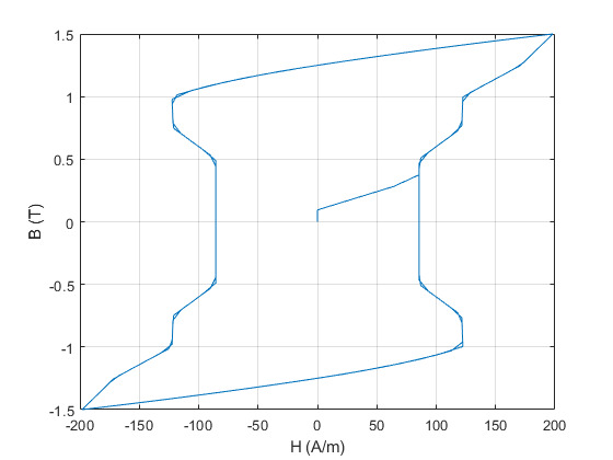
Plus, you can get really beautiful-looking hysteresis loops if you’re being me naive about it.

Next time

There you have it – some basic workings of the play and stop hysterons. Next time, we’ll take a look at

Losses with alternating excitation
Losses with rotating excitation
Generalizations
Whatever

Check out EMDtool - Electric Motor Design toolbox for Matlab.

Need help with electric motor design or design software? Let's get in touch - satisfaction guaranteed!

Stop Playing with Hysteresis