Magnetic levitation without 3D-FEA
Remember the earlier post about magnetic bearings? What about the principles of torque production in a typical electric motor with a relatively short airgap?
Unfortunately, neither of them will help you today, for we shall speak about maglev systems and how to model them analytically.
But first, let’s start with the basics, plus some motivational rah-rah.
What are maglev systems?
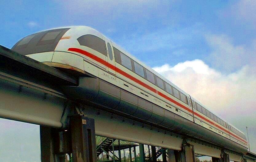
Maglev stands for magnetic levitation, simply. Although there are many applications, I’d wager that most people associate the term with the Japanese trains going really freaking fast. The reason they can do so is, well, levitation.
Actually, magnetic bearings are also a type of a maglev system. However, they are close to an electric motor in the sense that they typically feature iron cores combined with a small air gap. Moreover, they are based on magnetic attraction between two ferromagnetic pieces.
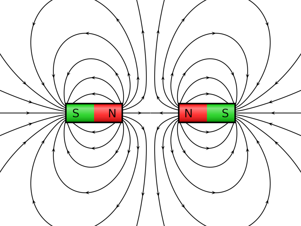
However, many maglev systems – the systems we are gonna speak about today – are pretty much the exact opposite. Instead of attraction, they are based on repulsion. You know, the kind you can actually feel when you try to push two magnets together, north-to-north.
Sidenote: the train-based systems seem to be based on either attraction between magnets, or repulsion due to eddy currents. But let’s focus on repulsion between magnets today.
Furthermore, the systems are typically air-cored. Meaning, there is no nice ferromagnetic path for the flux to follow. This is for a reason that might be obvious to some, and totally surprising to others (for me it can be both, depending on the day and my state of awareness). Namely, having an iron core would result in a reluctance force component. In other words, attraction of iron to a magnet – that’s what AMBs are usually based on. But now, we don’t want attraction – the system is based on repulsion now.
Complications
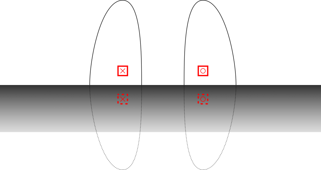
These two factors render our earlier analytical approaches more or less useless. Earlier, we could assume that the flux crosses the thin gap more or less perpendicularly. Thus, we could calculate it by simply dividing the linked current by the gap length.
But not anymore. There’s no gap, and the fluxes from the two opposing sources are bending out of their way to avoid each other. Thus, the assumption of nice straight flux lines doesn’t hold at all.
So what could help?
Obviously.
Published research and textbooks are always good bet. It’s pretty much certain you WILL find a nice formula for the repulsive force.
But let’s not go that way.
Understanding
There’s an inherent risk of using someone else’s result. You might be misunderstanding some definition, or neglecting some limitation that actually makes the nice formula invalid for your case. At the very least, you should try to derive the formula yourself to see if you understand the process.
One approach
So, how the approach the problem of air-borne fields? Again, the basics come in handy. Enter the Biort-Savart law.
The BS law (gotta love the name) let’s us nicely compute magnetic fields in vacuum or air. In mathematisque, it goes like this:
 .
.
Alright, it looks formidable, but it simply says that at any location  , the field is inversely proportional to the distance from the current (to the power of 2, to be exact).
Furthermore, it says that the contribution of any small piece of conductor  can be summed together separately. Hence the integration.
Finally, the field tends to circle around the current. Hence, the cross product.
Magnets
The BS law can be used to model magnets, too. Indeed, there are even two approaches for that, both based on certain little tricks.
The first is to replace the magnet by current sheet. This sheet would be placed on those outer surfaces of the magnet that are parallel to the magnetization direction. As can be visualized, it would in fact form a simple coil, generating a magnetic field in the same direction as the original magnet. Finally, the linear current density of this sheet would be equal to the magnet remanence flux density divided by its permeability. In other words, colossal. (This follows from the integral form of Ampere’s law – try it!)
The second approach is to use a fictitious magnetic charge on the north and south poles of the magnet. The magnetic field at any point can then be obtained from a modified Biort-Savart law
 .
.
As you can see, the volume integral over a conductor volume has been replaced by a surface integral around the magnet. The sigma symbol  denotes the fictitious magnetic charge density, equal to the dot product of the remanence flux density and the surface normal

Although this is perhaps even more unphysical than the current sheet approach, the results should be quite the same.
By the way, this Wikipedia article has some nice info on these two approaches.
Modelling iron components
The above approaches are very nice for anything air-cored. But what if were are analysing something else, that happens to have a back-iron for some reason? Like the attraction-based maglev system I mentioned earlier?
Well, in general – with saturating iron and complicated geometries – the situation is very complex. There, finite element analysis is your safest bet.
However, sometimes something simpler may suffice. For instance, if your iron can be reasonably approximated by an infinite sheet, the method of images can work nicely, also called the method of image charges.
Note: “an infinite sheet” might sound very unrealistic. However, that’s what you already do with the simple analytical models. Indeed, the airgap of an electric motor is usually so short that the curvature of the stator and rotor surfaces is negligible. In other words, both are modelled as infinite sheets.
Mirror charges
How mirror charges – or mirror currents, too – work, is quite easy.
First, you ignore the iron and treat everything as vacuum. Then, for any charge, you place another, fictitious charge inside the iron sheet. Its charge is either equal or opposite to the original (depending on the problem type), so that the resulting field crosses the iron boundary perpendicularly. Both charges are equally far from the surface – hence the term “mirror”.
The situation is a little more complex when you have two iron surface, like the stator and rotor of a machine. In this case, each charge is reflected from both surfaces. Furthermore, the mirrored charges are again reflected, as are their reflections, and so on.
Luckily, each additional reflection will be further away from the original. As the contribution of a charge drops quickly with distance (as is evident from the BS law, we only have to include a few to get decent-enough results. Remember that we are dealing with a quick approximate method in the first place – no sense to waste time on torturous mathematics the get the minor details _exactly_ right.
Forces
Alright, let’s finally get back to the original point: force computation. Luckily, it’s gonna be a short one.
With the current sheet method, the force is computed with the Lorentz force; the product of current and magnetic flux density. Short, see?
With the magnetic charge method…to be honest, I’m not sure really. (Plus I’m typing this on my mobile in the metro station, so I don’t wanna go through google-spewn pdfs at the moment.) But, I suppose it’s again an integral of the charge times flux density, equivalently to an electric charge in an electric field.
Alternatively, any of the standard methods can of course be used. For instance, the Maxwell stress tensor (or its weighted form) would certainly work.
Conclusion
An introduction to maglev systems. Or not really. More like a few approach to model the most common kinds of them. Educational, in other words.
Check out EMDtool - Electric Motor Design toolbox for Matlab.
Need help with electric motor design or design software? Let's get in touch - satisfaction guaranteed!